CGH 02

Where Do "Surface Maps" in Interferometers Actually Come From? — From a Set of Light-and-Dark Patterns to Surface Errors on the Test Piece

The "surface profile map" produced by an interferometer displays colors, variations in height, and a nanometer-scale grid. Yet, at the source—the detector—only patterns of light and dark are recorded. How, then, are surface irregularities derived from these variations in intensity?

In a CGH (Computer-Generated Hologram) null test, the nominal surface of the unit under test (UUT) is factored into the design of the test wavefront and the optical path geometry before any data is acquired. The height variations shown in the final map are determined not only by the phase of the light but also by this pre-established reference relationship.

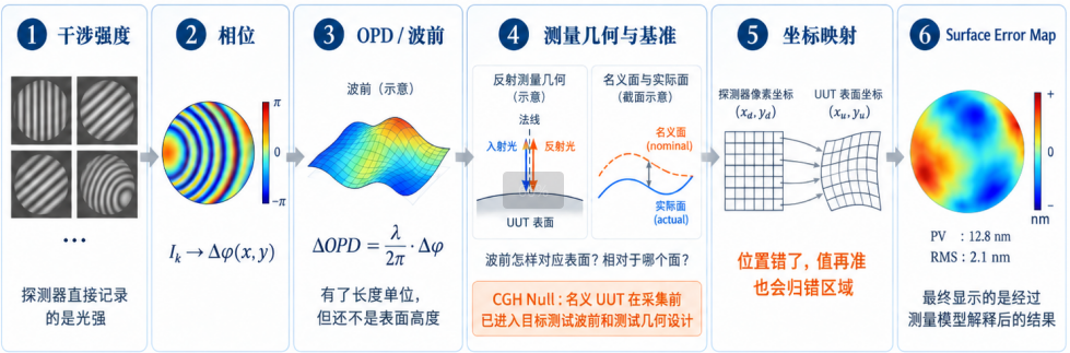
Figure 1 | From interference intensity to surface error: the relationships among numerical conversion, measurement geometry and references, and coordinate mapping.

I. Cameras record only light intensity—so where does the phase information come from?

When a reference beam and a test beam undergo coherent superposition on a detector, the phase difference between the two beams is encoded into the light intensity via an interference term. A camera records the brightness or darkness at each individual pixel, rather than the phase itself: [1]

While an image provides information on brightness and darkness, the intensity at each individual pixel cannot be directly equated to its phase. Phase-Shifting Interferometry (PSI) addresses this by introducing several known phase shifts and recording the intensity at each pixel across these different states.

For a given pixel—assuming the wavefront and light intensity remain stable and the frames are accurately registered—the intensity varies as a cosine function of the known phase shift. By analyzing this set of samples, the "wrapped" phase can be recovered for each pixel; this is then "unwrapped" by leveraging spatial continuity to restore the full-cycle phase values. However, phase unwrapping alone is insufficient to determine the absolute optical path length.[1,7]

Phase recovery establishes the phase difference between two light beams; to convert this into an optical path difference, a length scale—provided by the wavelength—is required.

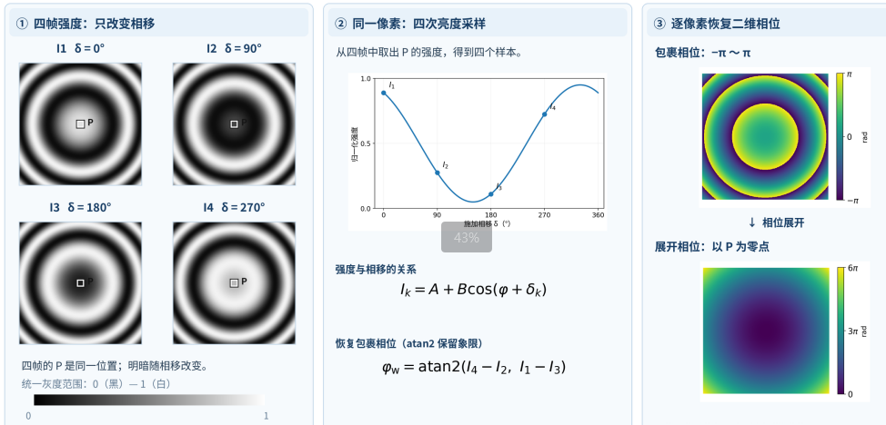
Fig. 2 | Four intensity frames are generated from the same phase field; the wrapped phase is then reconstructed from these intensities and subsequently unwrapped. P denotes a fixed pixel. This figure is generated based on a four-step calculation method and does not represent experimentally measured data. [7]

II. Given that the phase information is available, why can it still not be called a "surface profile"?

For monochromatic light, the wavelength establishes a scaling relationship between phase difference and optical path difference (OPD):

By converting the phase difference from radians into units of nanometers (nm) or micrometers (μm), the wavefront difference—or wavefront error—is assigned a linear scale. Although the units are now expressed in terms of length, the underlying physical quantity remains the optical path difference. This change in units does not transform the quantity into surface height.

To which propagation plane does this wavefront plot belong?

A 2D wavefront map is not a static map that simply translates along with the light beam. As a light beam propagates from one cross-section to another, its wavefront curvature and phase distribution evolve; therefore, in general:

The Hartmann method or lateral shearing interferometry first measures local slopes or phase differences, which are then used to reconstruct the wavefront at the measurement reference surface. When comparing these results with the design pupil (or exit pupil), it is necessary to account for the propagation plane or conjugate relationship; the sensor output cannot be directly equated to the wavefront at the exit pupil.[5,6]

In CGH-based null testing, the propagation position is also a design constraint. Upon reaching the specified location of the unit under test (UUT), the test beam must form a target wavefront that matches the ideal surface—meaning the local wave vector should align with the surface normal, with the light incident near-normally and returning along its original path.

This matching must hold true on the specific surface under test, rather than merely yielding a phase map with a similar appearance on an arbitrary cross-section.[2]

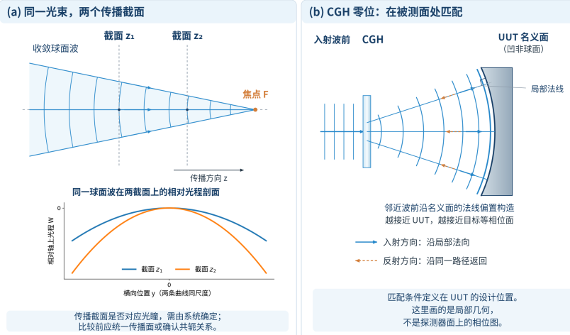
Fig. 3 | Left: Relative optical path profiles of the same converging spherical wave at two different propagation cross-sections, with uniform transverse and longitudinal scales; Right: The target wavefront of the computer-generated hologram (CGH) matched to the nominal surface at the design location of the unit under test (UUT). This is a schematic based on analytical geometry, not actual measured data.

III. From Wavefront to Surface: Why Is It Often Necessary to "Divide by 2" in Reflection-Based Measurements?

To transition from optical path difference to surface deviation, one must relate the change in optical path back to the reflection geometry. In air, for normal incidence, if a surface deviates by $\delta h_n$ along its local normal, a corresponding change in optical path occurs during both the incident and return paths. For small deviations—ignoring sign conventions—the first-order relationship is:

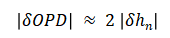
The familiar relation |δhₙ| ≈ |δOPD| / 2 arises from this round-trip optical path. The factor of "2" is determined by the measurement geometry; it is not a universal rule applied by the software to all reflection-based measurements.

When the incident light forms an angle θ with the local surface normal, the directional projection must also be accounted for when calculating the same deviation. Assuming the medium is air, a single reflection, and a small-deviation model:

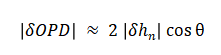
Here, θ represents the angle between the light ray and the local surface normal—not the tilt of the surface relative to the optical axis. Aspheric surfaces can be quite steep; however, under an ideal "null" test geometry, the test beam remains incident along the local normal of the nominal surface, keeping θ small.

The direction of the surface departure also factors into the conversion: in regions with steep slopes, the height difference measured along a fixed coordinate axis is not strictly equivalent to the deviation measured along the local normal of the nominal surface.

Furthermore, the measured residual wavefront may contain contributions from the reference optics, alignment, propagation, and the compensating elements themselves. Geometric conversion alone cannot isolate these individual sources; the converted result only acquires a clear, physically meaningful interpretation regarding the surface once these various contributions have been properly accounted for and the measurement geometry has been precisely defined.

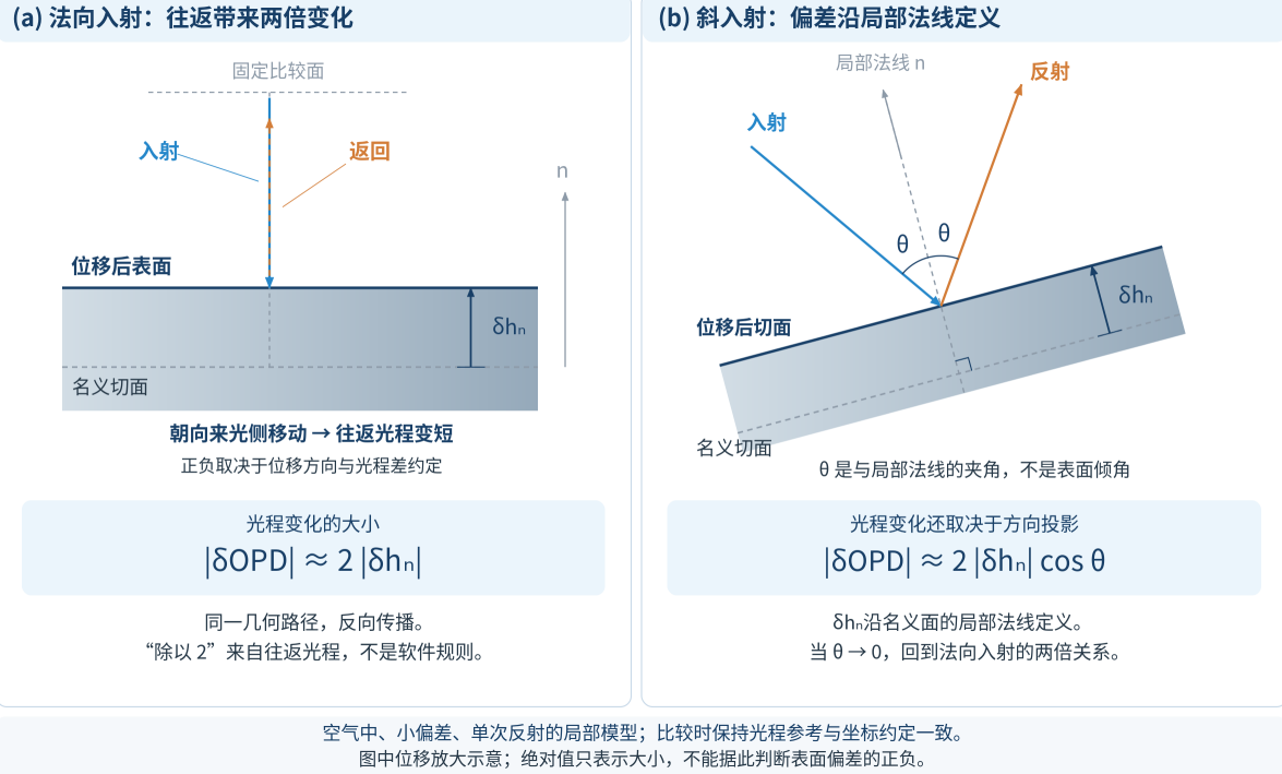
Fig. 4 | Optical path difference of reflected light versus normal displacement: left, normal incidence; right, local oblique incidence. The absolute value is used for the conversion, and the angle of incidence is defined with respect to the local normal.

IV. With respect to which surface is the surface-form error defined?

Surface error carries an additional implicit convention: it is always defined relative to a specific surface. The difference between an actual surface and its nominal design surface is termed a "departure from nominal"; once the permitted degrees of freedom for fitting are removed, the result is the "best-fit residual." While both can be visualized as color maps, they represent different concepts. Using a common coordinate system and a consistent height definition, this can be expressed as follows:

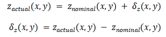
δz describes the deviation of the actual surface from the nominal surface and is used to evaluate manufacturing results; the aspheric departure from a reference/best-fit sphere describes the design surface itself. Since the comparison objects are different, the two departures are not the same quantity. The residual wavefront, however, still belongs to the measurement results under optical reference conditions and cannot be treated as surface deviation without conversion.

How can one participate in terms of nominal value?

While the comparison is always made against a nominal surface, the measurement approach can vary. Scanning 3D surface metrology—exemplified by the LUPHOScan system—obtains surface geometric information through multi-wavelength interferometric ranging combined with precise scanning-position metrology; the deviation from the nominal surface is then evaluated during the data-processing stage. This approach follows a "determine geometry first, then compare" logic.[3]

In contrast, CGH (Computer-Generated Hologram) null testing incorporates the nominal surface into the optical design prior to data acquisition. The target test wavefront and the test geometry are defined based on the nominal UUT (Unit Under Test). When the actual surface deviates from this nominal state, a residual wavefront is left in the returning light; through calibration, surface conversion, and coordinate mapping, the surface deviation relative to the nominal surface is ultimately derived.[2,4]

V. The numerical value has been calculated correctly—but where on the UUT does it correspond to?

A surface error map provides not only the magnitude of the deviation but also its specific location. While the aforementioned conversion explains the meaning of the "value," it does not automatically establish the corresponding "location."

The regular arrangement of pixels in the detector domain does not imply that the corresponding points on the surface under test (SUT) are equally spaced. In optical setups—such as those involving a transmission sphere, a null lens, or a computer-generated hologram (CGH)—non-linear imaging distortion may exist between the surface under test and the interferogram; this can be described by a coordinate mapping between the two domains.[1]

In the case of CGH-based testing, a regular sampling grid at the detector may not remain uniformly spaced when mapped onto the coordinate domain of the unit under test (UUT). Ignoring this mapping can lead to data values being assigned to the wrong regions of the surface. If the location is incorrect, even the most precise value becomes meaningless for that specific area. The coordinate mapping ensures that each measured value is correctly mapped back to its corresponding location on the UUT.[4]

The final displayed data may also undergo further processing, including the application of an effective aperture or mask, the handling of invalid data points, reference/calibration corrections, and the fitting and removal of terms such as piston, tilt, power, or other specific components. Processing sequences and available options vary between software packages; furthermore, applying different apertures or fitting criteria to the same raw dataset can result in different residual values in the final report.

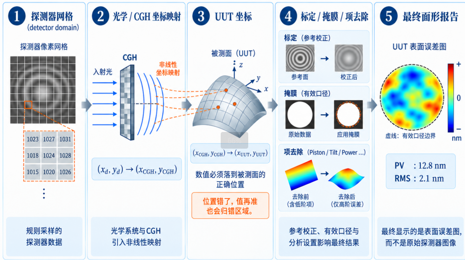
Figure 5 | From detector data to UUT surface error map

From Light and Shadow to Form

Intensity Frames → Phase Difference → OPD (Optical Path Difference) / Wavefront Error → Measurement Geometry & Reference → Coordinate Mapping → Surface Error → Final Report

The light and dark patterns initially captured by the camera are transformed—via phase retrieval—into an optical path difference (OPD). Through the application of measurement geometry, coordinate mapping, and reference conventions, this OPD is then interpreted as a surface deviation. Each step in this process alters not only the data format but also the physical significance represented by these numerical values.

Each value in the diagram is linked to both a surface location and a reference benchmark.The nanometer scale indicates the magnitude of a value, but it does not, by itself, specify what is being measured.

Next | From Design Phase to Microstructure: How Do CGHs Shape Test Wavefronts?

Appendix: Definitions and processing conditions for the results shown in the figures

References

[1] Ping Zhou. Error Analysis and Data Reduction for Interferometric Surface Measurements. Ph.D. Dissertation, University of Arizona, 2009. Focus on Chapters 1, 2, 3, and 5.

[2] Peng Jiantao. Research on Testing and Co-phasing Techniques for Large-Aperture Segmented Optical Systems Based on Computer-Generated Holography (CGH). Ph.D. Dissertation, University of Chinese Academy of Sciences, 2017. Focus on sections concerning CGH null compensation and test geometry.

[3] Taylor Hobson. LUPHOScan Non-contact 3D Optical Profilometer / MWLI technology; Best-fit methods for aspheres. Publicly available product and technical documentation.

[4] Arizona Optical Metrology (AOM). What is a CGH?; What is CGH mapping and how does it get corrected? Publicly available technical documentation.

[5] MathWorks. Model Shack-Hartmann Wavefront Sensor. See sections: "Shack-Hartmann Wavefront Sensor Principles" and "Measure Wavefront." https://www.mathworks.com/help/images/model-shack-hartmann-wavefront-sensor.html (Accessed: 2026-10-12)

[6] Phasics. Lens and assembly testing solutions. See section: "Single-pass measurement setup." https://www.phasics.com/en/applications/optics-systems-metrology/lens-and-assembly-testing/ (Accessed: 2026-10-12)

[7] Greg A. Smith. Phase Shifting Interferometry. University of Arizona. See sections: "Four Measurements" and "Final Comments." https://webs.optics.arizona.edu/gsmith/PhaseShift.html (Accessed: 2026-10-12)